How to Read a Forest Plot in a Meta-Analysis
META-ANALYSIS INTERPRETATION GUIDE
Examine the research question, effect scale, and null line before reviewing the diamond. Distinguish study point estimates, confidence intervals, statistical weights, pooled results, and prediction intervals without overinterpreting visual patterns.
A forest plot provides a compact graphical summary of a quantitative evidence synthesis. On a single axis, it displays individual study estimates, uncertainty intervals, statistical weights, subgroup divisions, and pooled results. While efficient, this density requires systematic reading. Visual position can easily be mistaken for clinical importance, marker size for study quality, or a pooled diamond for a universal finding that applies across all settings.
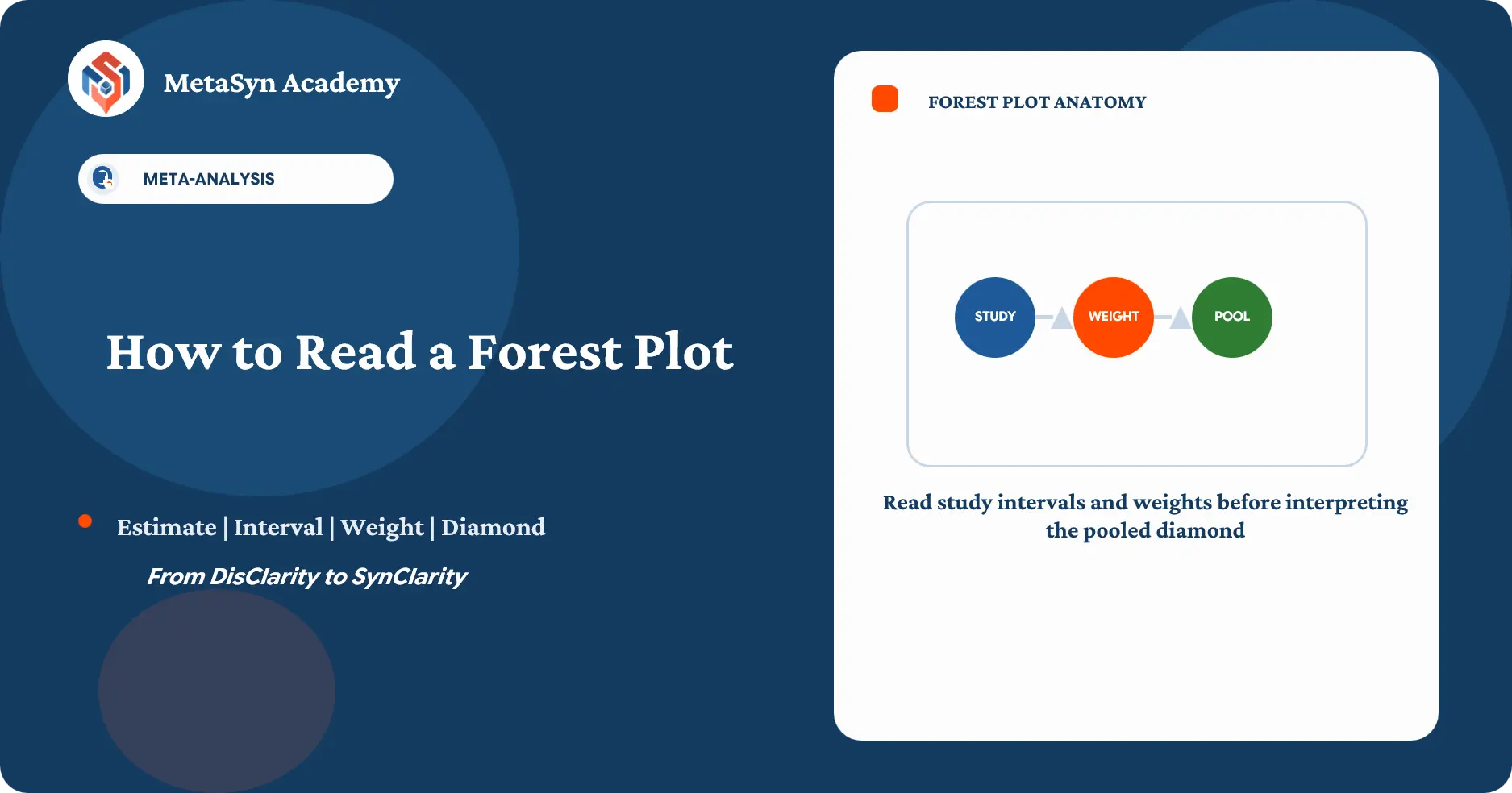
A structured reading sequence prevents common interpretation errors. First, identify the outcome, contrast, time point, effect measure, scale, null value, and direction. Next, evaluate each study estimate alongside its confidence interval. Then, review statistical weights and the pooled summary under the declared model. Finally, interpret heterogeneity, prediction intervals, and evidence boundaries. The original introduction of forest plots emphasized evaluating both individual studies and the synthesized summary together1; modern reporting demands the same systematic approach.
Use this actionable quality-control checklist to verify effect direction, scales, study weights, pooled estimates, and prediction intervals before publishing your review.
Explore the complete methodological framework for quantitative evidence synthesis, model selection, effect size transformations, and software reporting.
Access MetaSyn Academy’s central collection of downloadable worksheets, extraction forms, protocol logs, and reporting templates across all systematic review stages.
1. Confirm plot scope before reading results
Examine the title, outcome label, measurement timeframe, subgroup heading, comparison groups, and statistical model. Confirm whether the displayed figure reflects the primary analysis, a sensitivity check, or an exploratory subgroup. The number of plotted studies should match the evidence set described in the text. If a plot appears without its caption, consult the full report before drawing conclusions.
Forest plots are graphical summaries of an underlying data pipeline. The plot itself cannot verify whether eligible studies were grouped appropriately, whether correct data versions were extracted, or whether unit-of-analysis issues were addressed. Cochrane standards emphasize that study grouping and synthesis criteria must be established upstream of the graphical display6. When evaluating a review, verify the plot against the protocol, analysis scripts, and summary tables.
2. Identify the effect measure and its null value
The effect measure defines the mathematical scale of every point on the axis. Mean differences and standardized mean differences use zero as the null value representing no effect. Risk ratios, odds ratios, and hazard ratios use one as the null value. A risk ratio of 0.75 indicates that the event risk in the intervention group is 75% of that in the control group, which differs from a 25 percentage-point absolute risk reduction. Odds ratios must not be interpreted as risk ratios when outcome events are common.
Ratio measures are typically analyzed on a logarithmic scale and back-transformed for display. As a result, values of 0.5 and 2.0 appear equidistant from the null line of 1.0. Visual distance on a ratio plot cannot be translated into absolute differences without knowing baseline risk. Standardized continuous measures are expressed in standard deviation units, requiring context regarding scale direction, construct alignment, and clinical relevance.
Locate the vertical line marking the null effect and confirm it aligns with the chosen measure. Some plots include additional vertical lines for clinically meaningful thresholds or the pooled estimate. The figure legend must clarify these markers. Placing a null line at zero for a ratio measure or at one for a difference measure indicates a quality-control error.
3. Establish directional labels
Axis labels typically indicate which side favours intervention or control. Verify these positions carefully. For undesirable outcomes like mortality, lower values in the intervention group represent a favourable result. For desirable outcomes like recovery, lower values indicate an unfavourable result. Continuous instruments can also be scored in opposite directions across different studies.
Comparison order determines direction. Reversing intervention and control groups in a ratio inverted the value relative to one. Reversing groups in a mean difference changes its algebraic sign. A plot can appear visually coherent while carrying incorrect directional labels if group order or scoring conventions were misunderstood. Verifying a single study from raw data to its plotted location helps confirm accuracy.
4. Evaluate point estimates and confidence intervals
Each study entry features a central marker representing the point estimate and a horizontal line displaying the confidence interval. The marker indicates the calculated effect estimate from that sample. The confidence interval describes statistical precision under the chosen model, typically at a 95% level. Narrower intervals reflect greater statistical precision, while wider intervals indicate lower precision.
When a confidence interval crosses the null line, the study data remain statistically compatible with no effect at that confidence level. This does not prove that an intervention is ineffective. The interval may span both meaningful benefit and meaningful harm, indicating insufficient precision to draw conclusions. Conversely, excluding the null line demonstrates statistical incompatibility with zero difference, but it does not automatically confirm clinical importance or low risk of bias.
Arrows at the ends of a confidence interval signal that the range extends beyond the visible axis. Without these indicators, axis truncation can make estimates appear more precise than they are. Studies with zero events or sparse data require careful evaluation, as continuity corrections and variance adjustments can alter both point estimates and interval widths.
5. Interpret marker area and statistical weight
The area of the point estimate square corresponds to the study’s statistical weight in the synthesis. In a common-effect inverse-variance model, studies with smaller variance receive proportionally higher weight. In a random-effects model, estimated between-study variance is incorporated, which moderates differences among individual weights2.
Statistical weight differs from sample size. Event rates, variance estimates, allocation ratios, and model parameters all influence weight calculation. Importantly, weight does not reflect methodological quality. A large study with high risk of bias can exert substantial statistical weight, while a small, rigorous trial may receive little. Risk-of-bias appraisals must be evaluated separately from statistical weighting.
Reported weights within a meta-analysis should sum to approximately 100%. Visual square sizes should correspond proportionally to these values. Significant discrepancies between printed weights and marker areas indicate a graphical formatting error.
6. Read the pooled diamond summary
The midpoint of a diamond indicates the pooled point estimate, while its lateral tips mark the confidence interval. Certain software conventions use alternative shapes for subgroup totals or prediction intervals, making it necessary to confirm the legend. The pooled estimate reflects the chosen statistical model and interval method.
To evaluate a pooled diamond, first read the numerical estimate and interval bounds. Next, check whether the interval crosses the null line. Then, compare the range against established clinical thresholds to interpret the finding in absolute terms. Finally, contextualize the result using heterogeneity estimates, risk-of-bias evaluations, and certainty assessments.
A diamond that excludes the null line may reflect a small effect measured with high precision. Conversely, a diamond crossing the null line may encompass clinical benefit and harm. Statistical significance alone does not provide a complete summary. Cochrane guidance emphasizes evaluating effect magnitude, precision, variability, risk of bias, and evidence certainty together7.
7. Examine heterogeneity patterns
Heterogeneity represents variation in effect estimates beyond what would be expected from chance alone under a common-effect assumption. Evaluate the dispersion of point estimates, interval overlap, and clinical differences across studies before reviewing summary statistics. Similar point estimates can coexist with an influential outlier, while overlapping intervals may mask true variations in effect magnitude.
Cochran’s Q tests the statistical hypothesis that all studies share a single true effect. However, Q has limited statistical power when study counts are low and high power when syntheses include large samples. A non-significant Q test does not confirm homogeneity. $I^2$ measures the proportion of observed variance attributable to heterogeneity rather than sampling error. $I^2$ serves as a descriptive index of inconsistency rather than a strict model selector3.
$\tau^2$ estimates the between-study variance in a random-effects model, expressed on the scale of the effect measure. Because $\tau^2$ depends on the effect scale, its magnitude cannot be directly compared across different outcome measures. Heterogeneity statistics describe numerical variation; they do not explain whether variance stems from clinical diversity, methodological differences, or risk of bias.
8. Differentiate confidence intervals from prediction intervals
In a random-effects meta-analysis, the confidence interval around the pooled estimate reflects uncertainty regarding the mean of the underlying effect distribution. A prediction interval estimates the range of true effects expected in a new, comparable setting. A prediction interval can cross the null line even when the confidence interval around the mean does not, demonstrating that an average effect may not apply universally.
Calculating a prediction interval requires a plausible random-effects assumption and a sufficient number of studies to estimate between-study variance. With few studies, prediction intervals become imprecise. Plots should clearly label prediction intervals and state the calculation method. Prediction intervals should not be estimated informally from the spread of study point estimates, which includes sampling variation.
9. Evaluate subgroups and secondary diamonds
Forest plots displaying subgroup analyses often include summary diamonds for each category alongside an overall pooled estimate. Declaring a subgroup difference simply because one category summary excludes the null line while another does not is a common error. A difference in statistical significance between two groups does not confirm a statistically significant difference between them. Subgroup comparisons require a formal test for heterogeneity or interaction across groups.
Subgroup divisions are frequently observational and based on study-level characteristics, which may not reflect participant-level effect modification. Small subgroups can produce unstable estimates. Reviewers should verify whether subgroup analyses were prespecified, whether within-group pooling is methodologically sound, and whether proposed mechanisms are biologically or clinically plausible.
10. Avoid vote-counting
Counting the number of individual studies with confidence intervals excluding the null discards essential information regarding effect size and precision. A collection of small studies may each lack statistical power while their combined evidence provides a clear, precise summary. Conversely, multiple statistically significant studies can vary widely in direction or magnitude. Meta-analysis synthesizes estimates and uncertainty rather than tallying P-values.
Similarly, the visual proportion of study markers falling on one side of the null line does not substitute for a formal pooled calculation. Individual marker locations must be interpreted through study weights and precision. Always rely on the statistical synthesis, followed by a critical assessment of underlying assumptions.
11. Distinguish graphical results from risk of bias and certainty
Standard forest plots do not indicate whether studies used adequate randomization, allocation concealment, blinding, or complete outcome reporting. Incorporating traffic-light indicators into a figure can highlight risk of bias, but statistical weighting remains separate from methodological quality. A pooled estimate can be statistically precise while carrying a high risk of bias.
Certainty of evidence frameworks, such as GRADE, evaluate risk of bias, inconsistency, indirectness, imprecision, and publication bias. The pooled diamond represents the numerical synthesis; it does not assign an evidence grade. Findings from the forest plot feed into certainty assessments by defining effect magnitude, precision, and heterogeneity, while formal judgments belong in summary of findings tables.
12. Recognize publication bias boundaries
Although a pattern of smaller studies reporting larger effect sizes can raise questions, a forest plot cannot diagnose publication bias. Differences in study size can relate to study population, intervention dose, design features, or baseline risk. Funnel plots and formal regression tests assess small-study effects, though they carry specific application limits and cannot uniquely identify non-publication.
A balanced visual appearance on a forest plot does not rule out publication bias, as unpublished studies are absent from the display. Comprehensive literature searches, prospective registration reviews, and selective outcome evaluations are required to appraise publication bias thoroughly.
13. Worked reading example
Consider a forest plot of 12 randomized trials evaluating an intervention aimed at reducing a binary adverse outcome at 6 months. The chosen effect measure is a risk ratio, with intervention as the numerator. Values below 1.0 indicate a lower risk in the intervention group. The random-effects pooled risk ratio is 0.82 (95% CI: 0.68 to 0.99), with the confidence interval sitting just below the null line of 1.0.
An incomplete reading might simply conclude that the intervention is effective. A comprehensive reading notes that while the random-effects model indicates an 18% relative risk reduction on average, the upper confidence limit approaches 1.0. The reader then considers absolute baseline risk, clinical thresholds, risk of bias, variations in implementation, heterogeneity statistics, and the prediction interval. If the prediction interval spans from 0.55 to 1.22, the finding indicates that outcome effects vary across settings and may not be beneficial in every context.
14. Pre-publication quality control
| Category | Verification item | Common error |
|---|---|---|
| Identity | Confirm outcome name, timeframe, group contrast, and analysis dataset version. | Displaying an outdated figure alongside updated text. |
| Scale | Verify effect measure, axis transformations, tick marks, and null line position. | Interpreting log-transformed ratio axes as linear scales. |
| Direction | Check group assignment order, outcome coding, and directional axis labels. | Reversing “favours intervention” and “favours control” labels. |
| Study entries | Confirm study labels, numerical estimates, interval bounds, and subgroup placement. | Omitting an eligible study or duplicating an entry. |
| Weights | Verify printed weight values, visual marker sizes, and sum totals. | Treating statistical weight as a measure of study quality. |
| Summary | Confirm statistical model, pooled estimate, interval method, and diamond shape. | Plotted diamond values differing from summary text tables. |
| Heterogeneity | Verify Q, $I^2$, $\tau^2$, and associated calculation methods. | Applying threshold labels without clinical context. |
| Caption | Define abbreviations, confidence levels, models, and specialized symbols. | Leaving prediction intervals or subgroup totals unlabeled. |
When discrepancies appear, return to the raw dataset and analysis scripts. Correct the coding, re-run the synthesis, and regenerate the graphic. Manually editing plot labels or visual elements compromises reproducibility. Record revision details in project documentation.
15. Precise reporting language
Avoid reporting that “no effect was found” when a confidence interval crosses the null line. Instead, state that the estimate was imprecise and describe the range of compatible effects. Avoid stating that “all studies agreed” simply because point estimates share a common direction; describe differences in effect magnitude and precision.
Avoid describing a study with a large marker as the “highest quality” study. Clarify that it carried the largest statistical weight under the specified model. Avoid changing models solely because $I^2$ crossed an arbitrary threshold; model selection should reflect research questions and design assumptions. Finally, avoid concluding that an intervention is “clinically effective” based on a diamond alone, as clinical relevance depends on absolute risk reductions and patient-centered thresholds.
Master pre-specified synthesis planning, question framing, eligibility criteria, and PRISMA-P aligned protocol development before executing searches.
Navigate MetaSyn Academy’s complete step-by-step pathway from protocol registration and search design through statistical synthesis and GRADE assessment.
Verify your forest plot before reporting
Use our Forest plot interpretation and quality-control checklist to audit every graphic against your validated analysis output.
References
- Lewis S, Clarke M. Forest plots: trying to see the wood and the trees. BMJ. 2001;322(7300):1479-1480. doi:10.1136/bmj.322.7300.1479
- Deeks JJ, Higgins JPT, Altman DG, McKenzie JE, Veroniki AA. Analysing data and undertaking meta-analyses. In: Higgins JPT, Thomas J, Chandler J, et al., eds. Cochrane Handbook for Systematic Reviews of Interventions. Version 6.5. Cochrane; 2024:chap 10. Available from Cochrane
- Higgins JPT, Thompson SG, Deeks JJ, Altman DG. Measuring inconsistency in meta-analyses. BMJ. 2003;327(7414):557-560. doi:10.1136/bmj.327.7414.557
- Schild AHE, Voracek M. Finding your way out of the forest without a trail of bread crumbs. Res Synth Methods. 2015;6(1):74-86. doi:10.1002/jrsm.1125
- Page MJ, McKenzie JE, Bossuyt PM, et al. The PRISMA 2020 statement: an updated guideline for reporting systematic reviews. BMJ. 2021;372:n71. doi:10.1136/bmj.n71
- McKenzie JE, Brennan SE, Ryan RE, Thomson HJ, Johnston RV, Thomas J. Defining the criteria for including studies and how they will be grouped for the synthesis. In: Higgins JPT, Thomas J, Chandler J, et al., eds. Cochrane Handbook for Systematic Reviews of Interventions. Version 6.5. Cochrane; 2024:chap 3. Available from Cochrane
- Schünemann HJ, Vist GE, Higgins JPT, et al. Interpreting results and drawing conclusions. In: Higgins JPT, Thomas J, Chandler J, et al., eds. Cochrane Handbook for Systematic Reviews of Interventions. Version 6.5. Cochrane; 2024:chap 15. Available from Cochrane