
Heterogeneity in Meta-Analysis: Q, I², Tau² and Prediction Intervals
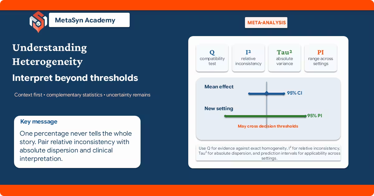
Heterogeneity is often compressed into a single percentage and an adjective: I2 was 72%, therefore heterogeneity was “high”. That sentence appears precise, but it leaves the principal scientific questions unanswered. Were the studies sufficiently compatible for an average to be meaningful? How far apart were the underlying effects on the analysis scale? How uncertain was the estimate of that dispersion? Did the variation cross a clinically or decision-relevant threshold? And which modelling assumptions produced the reported numbers?
Cochran’s Q, I2, the between-study variance τ2, its square root τ, and a prediction interval describe different aspects of the evidence. None identifies the clinical or methodological cause of variation, and none can decide by itself whether pooling is scientifically defensible. Their interpretation depends on the estimand, effect measure, study precision, number of independent studies, dependence structure, fitted model and intended decision.1–6
1. Heterogeneity begins with the estimand, not the statistic
Clinical diversity concerns differences in populations, interventions or exposures, comparators, outcomes, timing and settings. Methodological diversity concerns design, measurement, conduct and risk of bias. Statistical heterogeneity is the manifestation, within a specified model, of variation in observed effects beyond that expected from sampling error alone.1 Only the last of these is summarized by the familiar statistics. The first two determine whether the summary has a coherent scientific meaning and offer possible explanations for variation.
A random-effects analysis assumes that the studies estimate different but related underlying effects, conventionally represented by a distribution. Its summary is an estimate of the centre of that distribution. This changes the inferential target and the study weights; it does not correct risk of bias, eliminate heterogeneity or justify combining different estimands.1,12 When studies answer materially different questions, a structured synthesis without a pooled mean may be more defensible than an apparently sophisticated average.
2. Cochran’s Q: evidence against exact homogeneity
For a conventional inverse-variance meta-analysis, Cochran’s Q is a weighted sum of squared deviations of the study estimates from the common-effect estimate:
Under exact homogeneity and the usual large-sample assumptions, Q is compared with a chi-square distribution. A small p-value provides evidence that the observed differences are greater than expected from sampling error under that model. It does not quantify the magnitude, clinical importance or cause of heterogeneity. A non-significant result does not prove homogeneity, particularly when studies are few or imprecise; with many highly precise studies, the test may detect variation too small to matter substantively.1,2
3. I²: relative inconsistency, not an amount of heterogeneity
A conventional estimate of I2 is obtained by transforming Q:
I2 is commonly interpreted as the estimated proportion of variability in observed effect estimates that exceeds the variation expected from sampling error under the conventional model. It is not the percentage of studies that are heterogeneous, the probability that heterogeneity exists, the percentage by which effects differ, or an absolute measure of between-study dispersion.2–6
The statistic is precision-dependent. When within-study sampling variances become smaller while the absolute between-study variance remains unchanged, heterogeneity accounts for a larger share of total observed variability and I2 increases. Consequently, two reviews can have the same τ2 but very different I2 values. Cross-review rankings based on I2 alone are therefore misleading.4,6
Same between-study variance: τ² = 0.04
Relative share ≈ 20%Illustrative typical sampling variance = 0.16. Sampling error is large relative to the fixed between-study variance.
Same between-study variance: τ² = 0.04
Relative share ≈ 80%Illustrative typical sampling variance = 0.01. Sampling error is small relative to the same between-study variance.
Uncertainty is substantial when the evidence base is small. The point estimate can be biased upward or downward, and a confidence interval may span interpretations that would lead to very different substantive conclusions.5 Report uncertainty where the software and model support it, and avoid treating an estimate of 0% as proof of identical underlying effects.
The familiar descriptive ranges—0–40%, 30–60%, 50–90% and 75–100%—overlap deliberately and are explicitly qualified by the magnitude and direction of effects and the strength of evidence for heterogeneity.1 Likewise, the historically influential 25%, 50% and 75% labels were proposed as rough descriptors, not validated decision boundaries.3 Recent methodological reflection continues to emphasize that I2 measures inconsistency rather than absolute effect dispersion.6
4. τ² and τ: the absolute dispersion parameter
In the conventional random-effects model, τ2 is the between-study variance. It is expressed in squared units of the analysis scale. Its square root, τ, is the between-study standard deviation and is expressed on the analysis scale itself. Thus, when the model uses log odds ratios, τ is on the log-odds-ratio scale; when it uses a standardized mean difference, τ is in standardized-mean-difference units.1,7
Because τ shares the analysis scale, it is often more interpretable than τ2. Interpretation may still require back-transformation or comparison with a prespecified smallest effect size of interest. A value that appears numerically small can be decision-relevant on one scale and negligible on another.
| Estimator | Useful characteristics | Important limitations |
|---|---|---|
| DerSimonian–Laird | Simple, non-iterative and historically widespread. | Can underestimate heterogeneity and contribute to under-coverage in important configurations, especially when heterogeneity is appreciable or information is limited. |
| Restricted maximum likelihood | Often performs well across many continuous-outcome and general inverse-variance settings. | Remains uncertain with few studies, can estimate zero at the boundary and is not uniformly optimal. |
| Paule–Mandel | Often competitive across dichotomous and continuous-data simulations and closely linked to a generalized Q estimating equation. | Performance still depends on the data configuration; it should not be declared mandatory for an outcome type. |
| Maximum likelihood | Integrates naturally with likelihood-based modelling and model comparison. | May underestimate variance in small samples and should not be confused with REML. |
| Sidik–Jonkman-type estimators | Can perform well when heterogeneity is genuinely large. | May overestimate when true heterogeneity is small or moderate, depending on the implementation and starting value. |
No estimator removes the information limitation of a small meta-analysis. Point estimates of τ2 can differ substantially across methods, especially when the number of studies is low. The estimator, its uncertainty method, software implementation and non-default options should be reported together.7,8
5. Uncertainty around τ² is part of the result
A point estimate of τ2 is bounded below by zero and can equal zero even when substantively important heterogeneity remains plausible. Confidence intervals based on Q-profile, generalized-Q, profile-likelihood or other methods describe this uncertainty under different assumptions. Their coverage is approximate because sampling variances are estimated, random-effects assumptions may be imperfect and primary-study sample sizes may be limited.7,9,10
The appropriate conclusion is not that an interval including zero proves absence of heterogeneity, nor that an interval excluding zero establishes important inconsistency. Instead, interpret the range of plausible τ values on the analysis scale and ask whether that range permits effects that cross clinically or decision-relevant boundaries.
6. Confidence intervals and prediction intervals answer different questions
The confidence interval around a random-effects mean concerns uncertainty about the estimated centre of the distribution of underlying effects. It can be narrow even when the effects vary widely, particularly when many studies locate the mean precisely. A prediction interval incorporates estimated between-study dispersion and asks a different question: what range of underlying effects is compatible with a new study or setting judged exchangeable with those synthesized—or, more generally, what spread of underlying effects is permitted by the fitted model?1,11,12
The conventional prediction interval targets an underlying effect, not the noisy observed estimate that a future study would report. Predicting a future observed estimate would additionally require that study’s sampling variance. The interval also assumes that the new setting is sufficiently exchangeable with the included studies and that the random-effects distribution is appropriately specified.
Prediction-interval coverage can be poor when studies are few, study precisions are highly unequal or the assumed distribution of underlying effects is inappropriate. Different construction methods can yield materially different limits from the same data.11 Report the method, degrees of freedom or quantile, analysis scale, back-transformation and any warning generated by the software. In a large empirical reanalysis, prediction intervals frequently changed the practical interpretation obtained from the mean effect alone, illustrating why both summaries matter.13
7. Inference for the mean when studies are few
A conventional Wald interval treats the estimated between-study variance as sufficiently well determined and uses a normal critical value. This can produce confidence intervals that are too narrow when the number of studies is small. Hartung–Knapp–Sidik–Jonkman-type procedures use a t reference distribution and an adjusted variance estimate, often improving coverage in heterogeneous small meta-analyses.11,14
These methods are not uniformly superior. Unmodified Hartung–Knapp intervals can occasionally become unexpectedly narrow, particularly when the variance-adjustment factor is below one; modified procedures impose safeguards but can become very wide. Extreme imbalance in study precision and rare-event data remain difficult for all conventional methods.14,15 Wide intervals with two or three studies are often an honest representation of limited information rather than a software defect.
8. Dependence and software provenance are mathematical assumptions
Conventional formulas for Q, I2, inverse-variance random-effects models and their intervals generally assume independent effect estimates or a correctly specified covariance structure. Multiple outcomes, time points, subscales, treatment arms or reports from the same participants violate that assumption when entered as though they were independent. The usual consequence is overstated precision and potentially distorted heterogeneity estimates.16
Defensible options include selecting one prespecified effect per study, accounting for shared controls, specifying or estimating a covariance matrix, fitting multivariate or multilevel models, or using robust variance estimation with an appropriate small-sample correction. The number of independent study clusters should be distinguished from the number of effect estimates.
Software provenance is part of the statistical method. Record the program, package or module, version, function or command, effect transformation, τ2 estimator, mean-effect interval method, prediction-interval method, covariance assumptions, continuity corrections, zero-event handling and all non-default options. Method labels alone do not ensure that two programs implement identical calculations, and defaults can change over time.
9. Informative heterogeneity priors when the data cannot estimate τ² well
Bayesian random-effects models can incorporate external information about plausible heterogeneity through a prior distribution. Empirical predictive distributions derived from large collections of previous meta-analyses provide one principled source of such information, especially when the new synthesis contains too few studies to estimate τ2 reliably from its own data.17,18
This approach does not remove assumptions; it makes them explicit. The prior should correspond reasonably to the outcome type, intervention comparison and research context, and sensitivity analyses should show how conclusions change under alternative plausible priors. A prior borrowed from an unrelated evidence domain can be more misleading than an imprecise data-driven estimate.
10. Reporting heterogeneity without turning statistics into verdicts
PRISMA 2020 separates methods for exploring heterogeneity from the results of the synthesis and its investigations. Relevant reporting includes the synthesis model, effect measure, study count, summary estimate and precision, measures of statistical heterogeneity, results of heterogeneity investigations and all sensitivity analyses conducted.19,20 Completing a checklist or reporting I2 does not by itself establish PRISMA compliance or analytical validity.
A publication-ready heterogeneity statement should identify the estimand and analysis scale; report Q, degrees of freedom and p-value as a test of compatibility with exact homogeneity; report I2 with uncertainty as a relative descriptor; report τ2 and preferably τ with the estimator and uncertainty method; distinguish the mean-effect confidence interval from the prediction interval; and interpret all results against prespecified clinical or decision thresholds.
Prefer: “study effects varied beyond sampling error under the fitted model”; “the estimated between-study SD was … on the stated scale”; “the prediction interval crossed the prespecified no-effect or decision threshold”; and “the applicability of the average effect is uncertain across exchangeable settings.”
Related methodological articles and research tools
Meta-analysis heterogeneity interpretation worksheet
Document the estimand, pooling decision, data structure, Q, I², τ², τ, confidence intervals, prediction intervals and contextual conclusion.
Open the interpretation worksheet → Methodological overviewMeta-analysis heterogeneity, sensitivity analysis and publication bias
Examine how heterogeneity assessment connects with influence diagnostics, sensitivity analyses, small-study effects and missing-evidence judgments.
Read the methodological overview → Research templatesSystematic review and meta-analysis templates
Access evidence-informed worksheets, diagnostic logs, protocol-planning tools and reporting resources for systematic reviews.
Browse the research templates →Frequently asked questions
Why can two reviews have different I² values even when their absolute heterogeneity is similar?
Because I² is a relative, precision-dependent measure. The same between-study variance can account for a small share of total observed variability when studies are imprecise and a large share when studies are highly precise. Compare τ or τ² on the stated analysis scale, their uncertainty, the study effects and the prediction interval rather than ranking reviews by I² alone.4–6
Does a non-significant Q test show that the studies are homogeneous?
No. The Q test often has low power when studies are few or imprecise. A non-significant result means that exact homogeneity was not rejected at the sensitivity of the test under its assumptions; it does not prove that the underlying effects are identical.1,2
Which tau-squared estimator should I use?
No estimator is uniformly best. REML and Paule–Mandel often perform well across many conventional settings, while DerSimonian–Laird can perform poorly in some small or heterogeneous configurations. The choice should reflect the effect measure, study count, sparsity, balance of precision and model structure, and it should be reported with the software, version and uncertainty method.7,8
What does a prediction interval add beyond the confidence interval for the pooled mean?
The confidence interval describes uncertainty about the mean underlying effect. A prediction interval additionally incorporates estimated between-study dispersion and describes the range of underlying effects permitted for a new exchangeable setting under the fitted model. It is model-dependent and does not directly predict the observed estimate of a future study.11–13
Are fixed I² cutoffs valid rules for deciding whether to pool?
No. Published ranges are descriptive and overlapping, and their importance depends on effect direction, magnitude, uncertainty, absolute dispersion and clinical or methodological compatibility. The decision to pool should be based on the estimand and scientific coherence, not an I² threshold.1,3,6
Why can the same meta-analysis produce different results in different software?
Programs can differ in effect-variance calculations, default heterogeneity estimators, interval procedures, continuity corrections, optimization routines and handling of edge cases. Record the program, package, version, function, estimator, interval method, transformation and non-default settings so that another analyst can reproduce the result.
References
- Deeks JJ, Higgins JPT, Altman DG, McKenzie JE, Veroniki AA, et al. Chapter 10: Analysing data and undertaking meta-analyses. In: Cochrane Handbook for Systematic Reviews of Interventions. Current online version; chapter last updated November 2024. Cochrane. Accessed 4 August 2026. Available from: Cochrane Handbook Chapter 10.
- Higgins JPT, Thompson SG. Quantifying heterogeneity in a meta-analysis. Stat Med. 2002;21(11):1539–1558. doi:10.1002/sim.1186.
- Higgins JPT, Thompson SG, Deeks JJ, Altman DG. Measuring inconsistency in meta-analyses. BMJ. 2003;327(7414):557–560. doi:10.1136/bmj.327.7414.557.
- Borenstein M, Higgins JPT, Hedges LV, Rothstein HR. Basics of meta-analysis: I² is not an absolute measure of heterogeneity. Res Synth Methods. 2017;8(1):5–18. doi:10.1002/jrsm.1230.
- von Hippel PT. The heterogeneity statistic I² can be biased in small meta-analyses. BMC Med Res Methodol. 2015;15:35. doi:10.1186/s12874-015-0024-z.
- Higgins JPT, López-López JA. Reflections on the I-squared index for measuring inconsistency in meta-analysis. Res Synth Methods. 2026;17(3):389–402. doi:10.1017/rsm.2025.10062.
- Veroniki AA, Jackson D, Viechtbauer W, et al. Methods to estimate the between-study variance and its uncertainty in meta-analysis. Res Synth Methods. 2016;7(1):55–79. doi:10.1002/jrsm.1164.
- Langan D, Higgins JPT, Jackson D, et al. A comparison of heterogeneity variance estimators in simulated random-effects meta-analyses. Res Synth Methods. 2019;10(1):83–98. doi:10.1002/jrsm.1316.
- Viechtbauer W. Confidence intervals for the amount of heterogeneity in meta-analysis. Stat Med. 2007;26(1):37–52. doi:10.1002/sim.2514.
- van Aert RCM, van Assen MALM, Viechtbauer W. Statistical properties of methods based on the Q-statistic for constructing a confidence interval for the between-study variance in meta-analysis. Res Synth Methods. 2019;10(2):225–239. doi:10.1002/jrsm.1336.
- Partlett C, Riley RD. Random effects meta-analysis: coverage performance of 95% confidence and prediction intervals following REML estimation. Stat Med. 2017;36(2):301–317. doi:10.1002/sim.7140.
- Riley RD, Higgins JPT, Deeks JJ. Interpretation of random effects meta-analyses. BMJ. 2011;342:d549. doi:10.1136/bmj.d549.
- IntHout J, Ioannidis JPA, Rovers MM, Goeman JJ. Plea for routinely presenting prediction intervals in meta-analysis. BMJ Open. 2016;6:e010247. doi:10.1136/bmjopen-2015-010247.
- Röver C, Knapp G, Friede T. Hartung–Knapp–Sidik–Jonkman approach and its modification for random-effects meta-analysis with few studies. BMC Med Res Methodol. 2015;15:99. doi:10.1186/s12874-015-0091-1.
- Jackson D, Law M, Rücker G, Schwarzer G. The Hartung–Knapp modification for random-effects meta-analysis: a useful refinement but are there any residual concerns? Stat Med. 2017;36(25):3923–3934. doi:10.1002/sim.7411.
- Tanner-Smith EE, Tipton E, Polanin JR. Handling complex meta-analytic data structures using robust variance estimates: a tutorial in R. J Dev Life Course Criminol. 2016;2(1):85–112. doi:10.1007/s40865-016-0026-5.
- Turner RM, Davey J, Clarke MJ, Thompson SG, Higgins JPT. Predicting the extent of heterogeneity in meta-analysis, using empirical data from the Cochrane Database of Systematic Reviews. Int J Epidemiol. 2012;41(3):818–827. doi:10.1093/ije/dys041.
- Rhodes KM, Turner RM, Higgins JPT. Predictive distributions were developed for the extent of heterogeneity in meta-analyses of continuous outcome data. J Clin Epidemiol. 2015;68(1):52–60. doi:10.1016/j.jclinepi.2014.08.012.
- Page MJ, McKenzie JE, Bossuyt PM, Boutron I, Hoffmann TC, Mulrow CD, et al. The PRISMA 2020 statement: an updated guideline for reporting systematic reviews. BMJ. 2021;372:n71. doi:10.1136/bmj.n71.
- Page MJ, Moher D, Bossuyt PM, Boutron I, Hoffmann TC, Mulrow CD, et al. PRISMA 2020 explanation and elaboration: updated guidance and exemplars for reporting systematic reviews. BMJ. 2021;372:n160. doi:10.1136/bmj.n160.

